This article is about investigating an exponential signal and trying to model it using “simple” mathematical approach and a machine learning based approach.
In the day to day life of a scientist, most of the time we are invited by many forms of graphs. Some may represent the log phase of the growth of bacteria while others may represent a certain reaction cascading into faster rates over time.
We could also talk about the detection of electromagnetic waves after an explosive event such as a supernova. Whatever the case may be, we might come across some sort of noisy exponential graph. Note that this is just one example of a graph trend.
Other trends such as sigmoid, linear, logarithmic etc can also occur. For our purposes we are going to concentrate on an exponential graph.
Full codes for project are here.
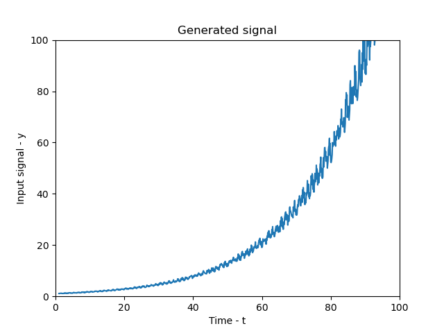
So let us dive into our investigation. The graph below shows a typical exponential noisy graph. Note that this was generated using a mathematical formula (all the code is included for the project) with a bit of random noise.
Method 1
In this method we are going to use a simple regression model, mathematically speaking. We realise that the law of our regression model could hold to be \(y = Ae^{Bx}\). In this case, we could linearize the equation then apply the Least Squares Method to find a system of normal equations.
Then using a few selected data values for \(x\) and \(y\) we can perform the regression. However this is long and tedious! We could make use of the technology already available to us and use some online regression calculators. For our purpose, we can use this calculator to find the values of \(A\) and \(B\).
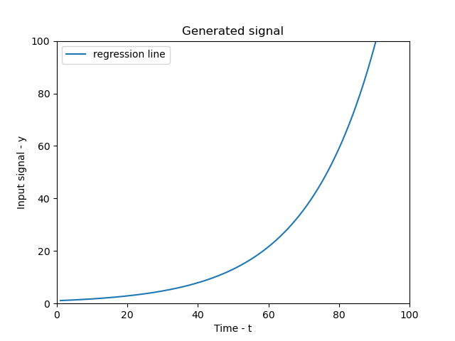
We are going to input the first 20 data values from our dataset (dataset is included in the project folder). We get our values as \(A=1.057826806\) and \(B=0.0502770095\). Using these values, we get the following graph.
Comparing this to our actual dataset, we have…
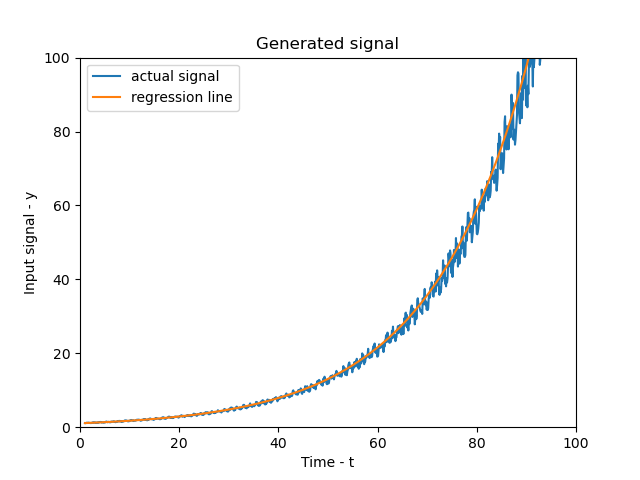
Not too bad considering it’s a curveof best fit! It wouldn’t give us the most accurate results but it’d be a good estimate for predicting the values on the go using lower computer resources. Now let us consider the second method
Method 2
Let us use the most popular method used by data scientists nowadays. Machine Learning approach. In this approach we are going to use a multi-layer perceptron model to predict the signal. Firstly we can see that our previous method used a simple mathematical regression and it gave us a curve of best fit. However,
in that approach it couldn’t mimic the “random noise” that was present in our signal. So an inspiration that we can take is from time series forecasting. In time series forecasting method, it takes into account the cyclic behaviour of a data and also sudden dips and ups. Hence using a multilayer perceptron regression (instead of simple regression) to do time-series forecasting is our preferred method. An excellent tutorial for this can be found here.
Using our model, we achieve the following results.
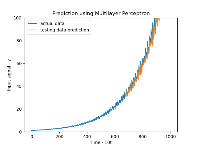
The results are simply too good! It’s able to account for the periodic ups and downs in the data and does a far better job at predicting the values.
Conclusion
As we can see that using a normal naive mathematical model doesn’t quite produce realistic results because more often then not, they seem to be “too perfect”. However it is useful when estimations are needed to be done fast. Mathematical models rather may be used to study a pattern over long term rather than being precise for shorter periods of time.
We can see that using the advancments in the field of machine learning and artificial intellingence, we are better able to model realistic situations and behaviours. ML and AI are thechnically mathematical models in essence, but that’s a topic for another day…